Optimization

Intent

In this blog, post I will cover different approaches for gradient-free optimization. The main focus will be on Bayesian Optimization and in order to understand Bayesian Optimization, we will cover Gaussian processes.

In full transparency, my original intent for the post was to show for a real-world example that random grid search was just as good as Bayesian optimization. However, keeping the number iterations between the two methods Bayesian optimization found a better solution. This came at the cost of computation time. The Bayesian optimization method was significantly slower. This once again reminds me that in data science there are no perfect models or solutions. Every approach has it’s advantages and disadvantages.

Hopefully, this post can at least provide you with an appreciation of what is going on behind Bayesian optimization.

Introduction

Optimization appears throughout machine learning and in many different forms. Mathematically speaking, optimization is the process of maximizing (or minimizing) a real function by choosing inputs values, in some systematic way, from a defined set. In other words, we want to find the parameters that will give us the best outcome.

Traditionally, we think about optimization in terms of training a model. In this case, we are using optimization to find the parameters \(\theta\) of a model that minimizes the cost function \(J\left(\theta\right)\). The great thing about this optimization is that we have a guide to help us minimize or maximize the cost function. This is the first derivative of the cost function \(\frac{\partial}{\partial \theta}J\left(\theta\right)\). In gradient descent, the first derivative is a guide that tells the optimization where to look for the minimum (or maximum) of the function.

\[\theta^{\prime} = \theta - \alpha \frac{d}{d\theta}J\left(\theta\right)\]

where \(\theta^{\prime}\) is the updated version of \(\theta\) and \(\alpha\) is the learning rate which dictates how much large the steps we take in updating the parameter \(\theta\).

We add a layer of complexity to model training when we search for the optimal hyper-parameters to use for a model. For each set of hyper-parameters that we try, we have to train a model. Finding the best hyper-parameters is another type of optimization problem. Now we have layered optimizations. In the first layer, training the model, we have a clear cost function that is differentiable by the model coefficients (parameters). This guide helps us find the best fit model.

In the outer layer, the parameters that we are trying to optimize exist outside of the cost function. Therefore, in most cases, we can not compute the partial derivatives of the hyper-parameters with respect to the cost function. There are techniques to try to determine the gradients for hyper-parameters but they are difficult to implement (Franceschi et al., 2017; Maclaurin et al., 2015). Imagine you are in a new city trying to find a restaurant and the GPS and maps functionality stop working on your phone. Even though we no longer have a guide, we can still search for our restaurant randomly or in a systematic fashion.

Hyper-parameter optimization is not the only type of optimization we can do. Say, for example, we build a model to predict the strength of steel based on manufacturing parameters such as the temperature of furnace and amount of iron ore and carbon. We can utilize optimization to find the best combination of temperature, iron ore, and carbon to give us the strongest steel. In this case, our objective function (what we want to maximize) is the actual model itself and we can neither write an analytical expression for this nor take its partial derivatives. This example and the hyper-parameter tuning are both cases where don’t have a guide or a gradient to follow.

Grid Search and Random Search

Two relatively straight forward ways to conduct gradient-free optimization is grid search (systematic) and random search (random). In grid search, we partition the hyper-parameter space and systematically evaluate points within the space.

*Figure 1. Representation of grid search where each blue dot represents a point in parameter space to evaluate the model.*

Grid search is systematic in that we search through all possible combinations of hyper-parameters. Say for example we have the hyper-parameters \(\alpha\), \(\beta\), and \(\gamma\) and each parameter has 100 different values that we would like to explore. This leads to a total of \(1,000,000\) different combinations to explore and for each combination, we must build a new model. Computationally, this is very expensive!

With random search, we can take a random sampling of all the possible combinations of parameters. How many combinations we evaluate depends on our appetite for model training time. We could randomly sample \(100\) or \(1,000\) or even \(100,000\) of the total \(1,000,000\) combinations. The hope is that we sample a point close to or at the global minimum of our cost function.

*Figure 2. Representation of random grid search where each blue dot represents a point in parameter space to evaluate the model.*

Bayesian Optimization

As we evaluate points in our search, wouldn’t it be cool if we could somehow incorporate the information we learned from previous points in our parameter space to guide us where to look next? Hmmmm, this sounds suspiciously Bayesian.

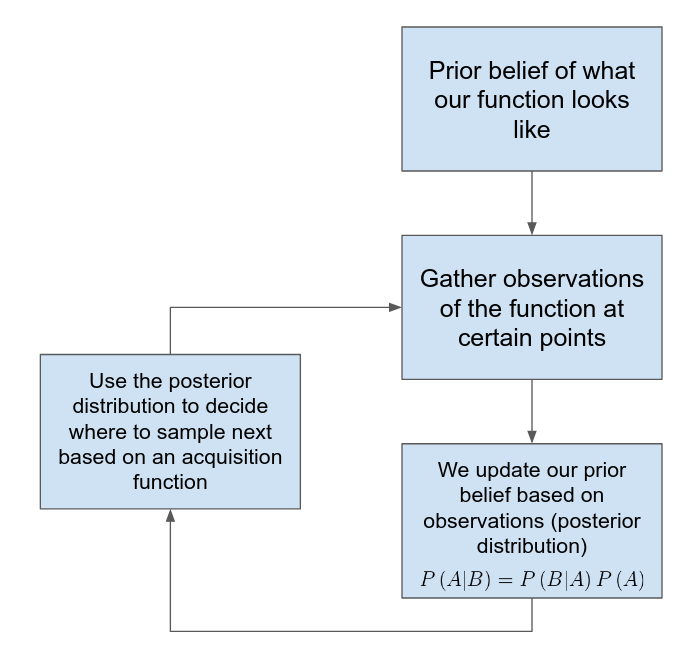
How does Bayesian optimization work?

We model our function, \(f\), as a probability distribution (surrogate model)
When we compute \(f\) at parameter values \(x_{1}, x_{2}, ..., x_{N}\), we consider \(f\left(x_{1}\right), f\left(x_{2}\right), ..., f\left(x_{N}\right)\) to be observed variables in the model
These observations update our prior belief of what \(f\) looks like and help us decide where to evaluate the function next

*Figure 3. Flow chart showing steps for Bayesian Optimization.*

Gaussian Processes (GP)

One way to define our surroget model is to us Gaussian processes (GPs). With a traditional linear regression type problem we fit the parameters to a specific function using something like Least Squares. Gaussian Process is different from this method in two major ways:

GP in non-parametric. Rather than solving for a finite set of parameters of a specific function we look for a distribution of functions over infinitely many parameters
With GP we can update the distribution of functions everytime we observe a new data point (training data). In other words we construct a prior distribution (over functions) and update the distrubtion by conditioning on data.

Let’s walk through Gaussian Proccesses at a high level to gain intuition. For a more mathematical approach check out Kevin Murphy’s book Machine Learning: A Probablistic Perspective and Görtler et al, 2019.

In the traditional approach to regression problems, we restrict ourselves to a class of functions and look for the parameters which make that function best fit the data. In the GP approach, we describe a probability over all possible functions and previous observations help give us an idea of which functions are more likely. There is beauty and impracticality in this perspective. How does one evaluate an infinite number of functions? The idea of infinite functions is a level of abstraction. We don’t need to specify each each individual function. We only need to define the distribution

The goal of GP is to learn the distribution of functions given the training data

\[p\left(f\lvert X, y \right)\]

Where \(f\) represents a continuous function and \(X\) is our training data.

It’s worth mentioning that Gaussian distributions are closed under conditioning and marginalization. Closed under marginalzation means that when can isolate one part of a multivariate Gaussian distribution and that part will also be Gaussian. Because of this property we can easily focus on specific positions of the function that we have observational data for and ignore the rest.

Closed under conditioning means that we can determine the probability of one variable (also Gaussian) conditioned on another variable. This property allows us to use Bayesian inference or update our prior distribution with data to create a posterior distribution.

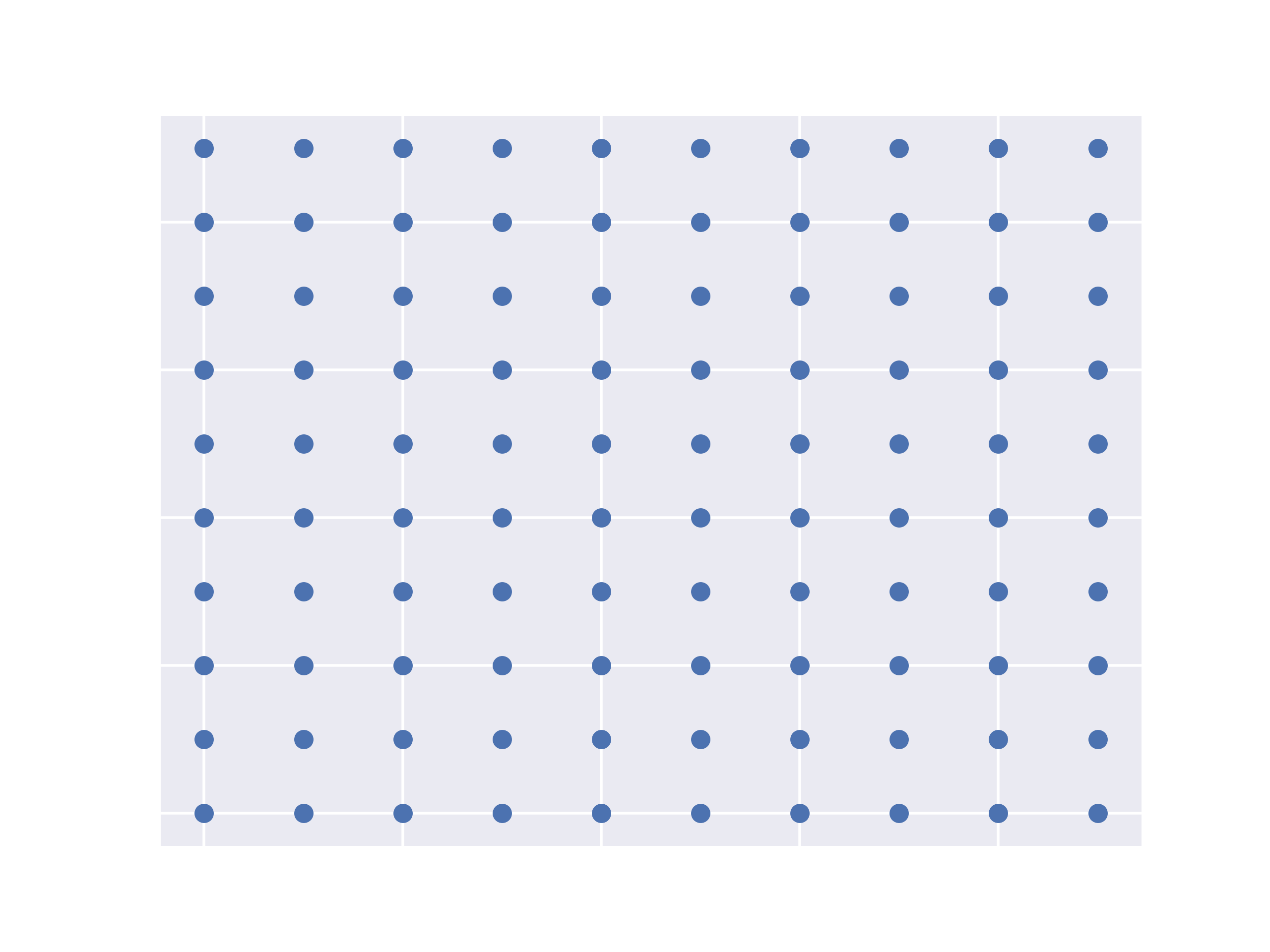
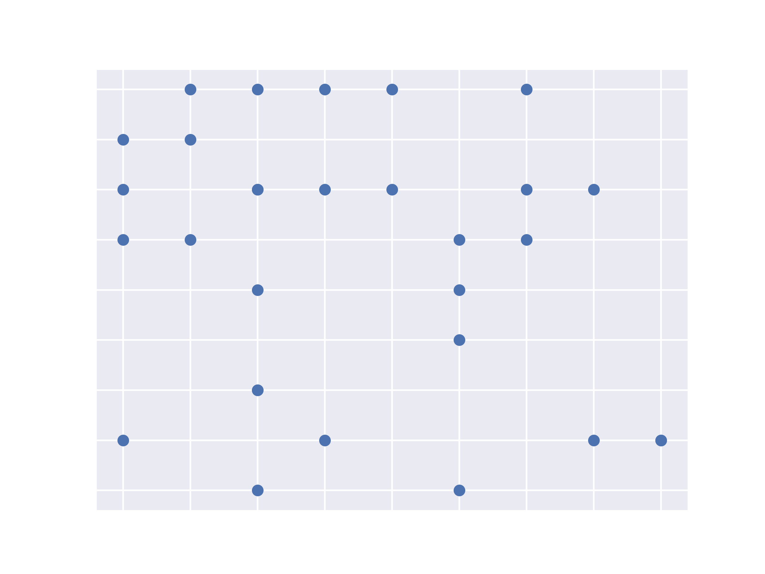
Although we are fitting over functions it will serve us well to shift our perspective from that of a continuous function to discrete representation of a function (i.e. what is the value of the function at a certain point). This is important because we will be sampling points from the Gaussian distribution to make predictions.

import numpy as np
from sklearn import gaussian_process
from sklearn.gaussian_process.kernels import RBF, ConstantKernel as C
from sklearn.gaussian_process import GaussianProcessRegressor

# ---------------------------------------------------------
# This is the actual function that we would like to predict
# ---------------------------------------------------------
f = lambda x: np.sqrt(x) * np.sin(x)

# -----------------------
# x-values for evaluation
# -----------------------
x = np.atleast_2d(np.linspace(0, 10, 1000)).T

# ----------------------------------
# Instantiate Gaussian process model
# ----------------------------------
# Define Kernel (Covarience matrix)
kernel = C(3.0, (1e-3, 1e3)) * RBF(10, (1e-2, 1e2))
gp = GaussianProcessRegressor(kernel=kernel, n_restarts_optimizer=9)

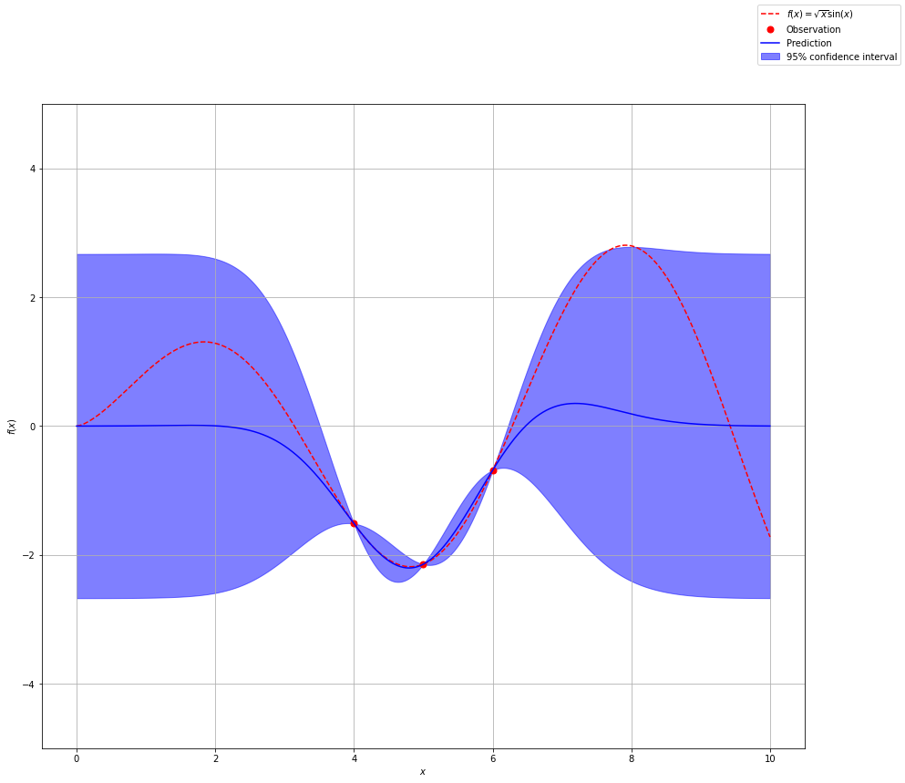
So far we have not added any observations to update our prior belief. Therefore our current best guess (posterior) spans all of the possible functions.

import matplotlib.pyplot as plt


y_pred, sigma = gp.predict(x, return_std=True)

fig, ax = plt.subplots(figsize=(15, 13))
ax.plot(x, f(x), '-r', label=r'$f(x) = \sqrt{x}\sin(x)$')
ax.plot(x, y_pred, 'b-', label='Prediction')
ax.fill_between(
    x.flatten(), 
    y_pred.flatten() + 1.96 * sigma.flatten(), 
    y_pred.flatten() - 1.96 * sigma.flatten(), 
    alpha=0.5, 
    color='b', 
    label='95% confidence interval'
) 
ax.set_xlabel('$x$')
ax.set_ylabel('$f(x)$')
ax.set_ylim(-5, 5)
ax.grid(True)
fig.legend()
plt.show()

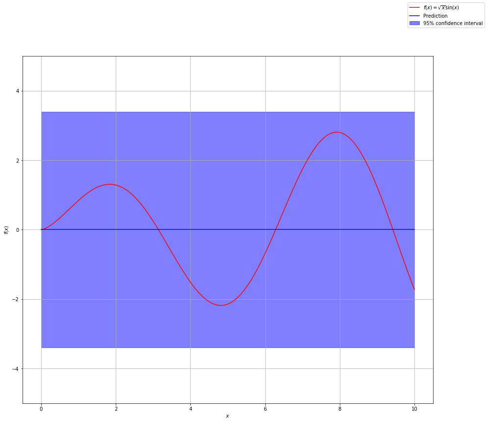
*Figure 4. The red line indicates the actual function we wish to estimate. The blue shaded region represents the distribution of all functions within our confidence bounds.*

The dark blue line represents the mean of all possible functions we are considering. Remember our distribution spans an infinite number of functions. There are infinitely many functions that could fit the data. For predictions, we use the mean of these functions. The shaded blue area represents the confidence in our prediction. We get this from the standard deviation of each point which comes from the covariance matrix of the implied Gaussian distribution.

Now let’s start adding some observational data. This is our training data that will help inform our prior distribution (which right now is pretty much everything). Let’s see what happens if we add two data points.

gp = GaussianProcessRegressor(kernel=kernel, n_restarts_optimizer=9)
x_obs = np.array([4, 5, 6])
y_obs = f(x_obs)

x_obs = np.atleast_2d(x_obs).T
y_obs = np.atleast_2d(y_obs).T

gp.fit(x_obs, y_obs)

y_pred, sigma = gp.predict(x, return_std=True)

fig, ax = plt.subplots(figsize=(15, 13))
ax.plot(x, f(x), '--r', label=r'$f(x) = \sqrt{x}\sin(x)$')
ax.plot(x_obs, y_obs, '.r', markersize=14, label='Observation')
ax.plot(x, y_pred, 'b-', label='Prediction')
ax.fill_between(
    x.flatten(), 
    y_pred.flatten() + 1.96 * sigma.flatten(), 
    y_pred.flatten() - 1.96 * sigma.flatten(), 
    alpha=0.5, 
    color='b', 
    label='95% confidence interval'
) 
ax.set_xlabel('$x$')
ax.set_ylabel('$f(x)$')
ax.set_ylim(-5, 5)
ax.grid(True)
fig.legend()

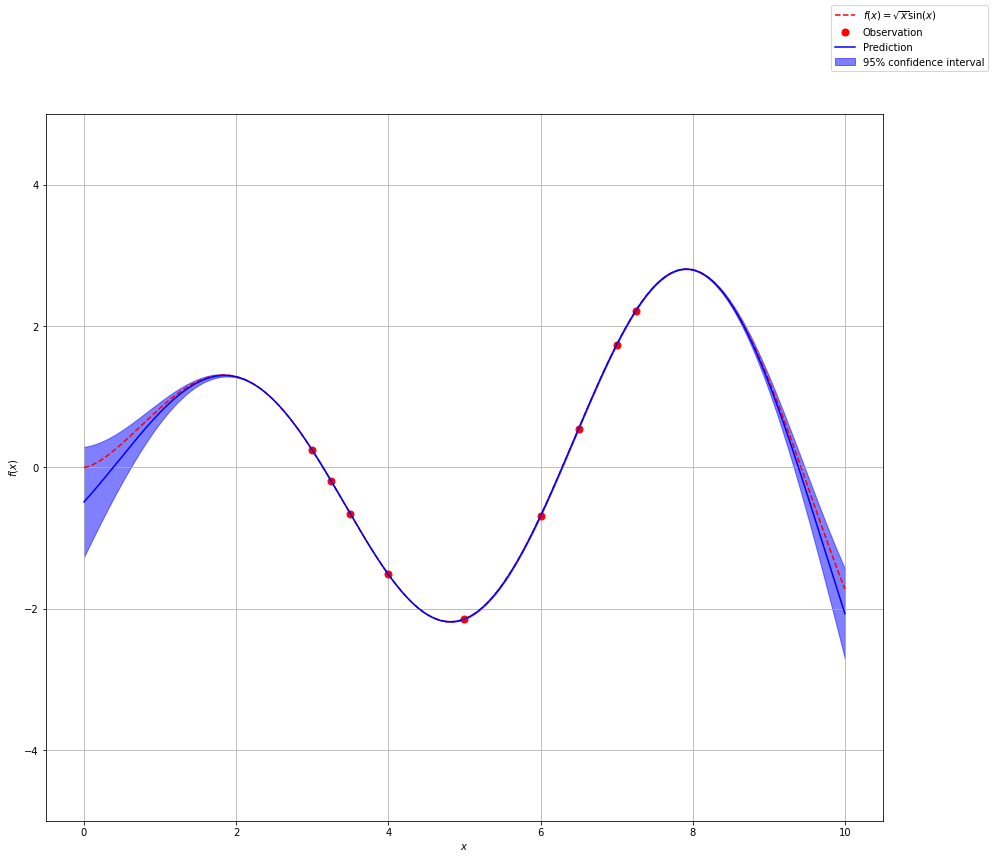
Figure 5. The dashed red line indicates the actual function we are trying to estimate. The red dots indicate points we have sampled at. The blue line is the mean of the distribution of functions we are considering.

Notice how we have more confidence around our observations and as we move further from our observations we are less confident in our prediction. Let’s add a couple of more data points.

gp = GaussianProcessRegressor(kernel=kernel, n_restarts_optimizer=25)
x_obs = np.array([3, 3.25, 3.5, 4, 5, 6, 6.5, 7, 7.25, ])
y_obs = f(x_obs)

x_obs = np.atleast_2d(x_obs).T
y_obs = np.atleast_2d(y_obs).T

gp.fit(x_obs, y_obs)

y_pred, sigma = gp.predict(x, return_std=True)

fig, ax = plt.subplots(figsize=(15, 13))
ax.plot(x, f(x), '--r', label=r'$f(x) = \sqrt{x}\sin(x)$')
ax.plot(x_obs, y_obs, '.r', markersize=14, label='Observation')
ax.plot(x, y_pred, 'b-', label='Prediction')
ax.fill_between(
    x.flatten(), 
    y_pred.flatten() + 1.96 * sigma.flatten(), 
    y_pred.flatten() - 1.96 * sigma.flatten(), 
    alpha=0.5, 
    color='b', 
    label='95% confidence interval'
) 
ax.set_xlabel('$x$')
ax.set_ylabel('$f(x)$')
ax.set_ylim(-5, 5)
ax.grid(True)
fig.legend()

Bayesian Optimization

Gaussian processes are the foundation for Bayesian Optimization. For Bayesian Optimzation we are not necessarily trying to fit the entire function, rather we are trying to find the global maximum or minimum of the function within our parameter space.

We use Gaussian Process to develop a form of the function we are looking for. In our previous examples we just randomly chose observations to constrain our function. With Bayesian Optimization we want some sort of smart algorithm to help guide where we next evaluate the function.

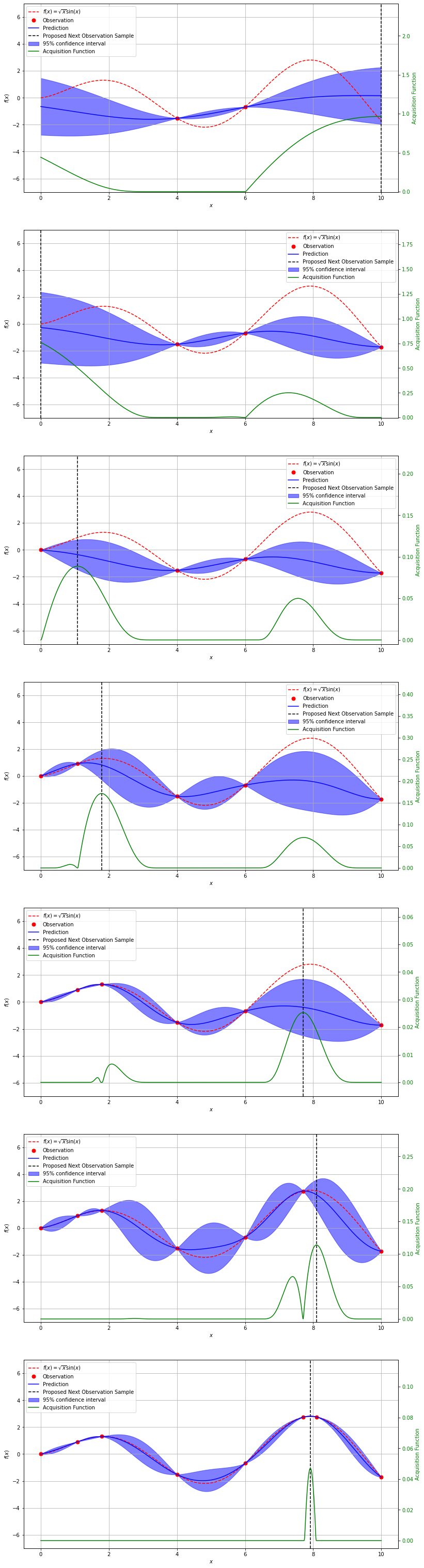
With Bayesian optimization, we introduce two new terms, surrogate model and acquisition function. The surrogate model comes from Gaussian Process and is the mean of our posterior distribution over functions. The aquisition function is something new. It will help guide use to the next point we should evaluate.

The acquisition function is a trade off of exploration versus exploitation. Exploitation means that we want to quickly find a maximimum or minimum point guided by our current observations. This is done by looking at points where the surrogate function is high (maximum) or low (minimum). Exploration means that we want to explore the entire space to make sure that we find the global minimum or maximum. Areas with large confidence intervals have the most uncertainity, therefore, if we explore that space we will gain the most information. The acquisition function will balance exploration and exploitation.

from scipy.stats import norm

def expected_impr(X, X_sample, Y_sample, gpr, xi):
    mean, std = gpr.predict(X, return_std=True)
    std = std.reshape(-1, X_sample.shape[1])
    
    y_max = np.max(gpr.predict(X_sample))
 
    with np.errstate(divide='warn'):
        a = (mean - y_max - xi)
        z = a / std
        ei = a * norm.cdf(z) + std * norm.pdf(z)
        ei[std==0.0] = 0.0

    return ei


from scipy.optimize import minimize
from functools import partial


def aquisition_max(acquisition, X_sample, Y_sample, gpr, bounds, n_restarts=25, xi=0.01):

    dim = X_sample.shape[1]
    max_acq = None
    
    x_seeds = np.random.uniform(bounds[:, 0], bounds[:, 1], size=(n_restarts, dim))
    for x0 in x_seeds:
        res = minimize(lambda x:-acquisition(x.reshape(1, -1), X_sample, Y_sample, gpr, xi), 
                       x0=x0, bounds=bounds, method='L-BFGS-B')        
        if max_acq is None or -res.fun[0] >= max_acq:
            max_acq = -res.fun[0]
            x_max = res.x           
            
    return np.clip(x_max.reshape(-1, 1), bounds[:, 0], bounds[:, 1])

Now with our aquisition function defined, we can walk through the process of finding the maximum of our previous function. You will see that the maximum of our aqusition function tells us where to sample next.

gp = GaussianProcessRegressor(kernel=kernel, n_restarts_optimizer=9)
np.random.seed(42)

# ---------------
# Initial samples
# ---------------
x_obs = np.array([4, 6])
y_obs = f(x_obs)

x_obs = np.atleast_2d(x_obs).T
y_obs = np.atleast_2d(y_obs).T

# -----------------------------
# Number of observations to try
# -----------------------------
n_obs = 7
bounds = np.array([[0, 10]])

fig, ax = plt.subplots(n_obs, figsize=(13, 55))

# Loop through observations
for i in range(n_obs):

    # Update the surroget model with new observations
    gp.fit(x_obs, y_obs)

    y_pred, sigma = gp.predict(x, return_std=True)

    # Use the acquisition function to find the next value to sample
    x_next = aquisition_max(expected_impr, x_obs, y_obs, gp, bounds)
    y_next = f(x_next)

    acq_vals = expected_impr(x, x_obs, y_obs, gp, xi=0.01)

    # Plot
    ax[i].plot(x, f(x), '--r', label=r'$f(x) = \sqrt{x}\sin(x)$')
    ax[i].plot(x_obs, y_obs, '.r', markersize=14, label='Observation')
    ax[i].plot(x, y_pred, 'b-', label='Prediction')
    ax[i].fill_between(
        x.flatten(),
        y_pred.flatten() + 1.96 * sigma.flatten(),
        y_pred.flatten() - 1.96 * sigma.flatten(),
        alpha=0.5,
        color='b',
        label='95% confidence interval'
    )
    ax[i].axvline(x_next, color='k', linestyle='--', label='Proposed Next Observation Sample')
    ax2 = ax[i].twinx()
    ax2.plot(x, acq_vals, '-g', label='Acquisition Function')
    ax2.tick_params(axis='y', labelcolor='g')
    ax2.set_ylim(-0.005, 2.5 * np.max(acq_vals))
    ax2.set_ylabel('Acquisition Function', color='g')
    ax[i].set_xlabel('$x$')
    ax[i].set_ylabel('$f(x)$')
    ax[i].set_ylim(-7, 7)
    ax[i].grid(True)
    
    x_obs = np.vstack((x_obs, x_next))
    y_obs = np.vstack((y_obs, y_next))

    h1, l1 = ax[i].get_legend_handles_labels()
    h2, l2 = ax2.get_legend_handles_labels()

    ax[i].legend(h1 + h2, l1 + l2, prop={'size':10})

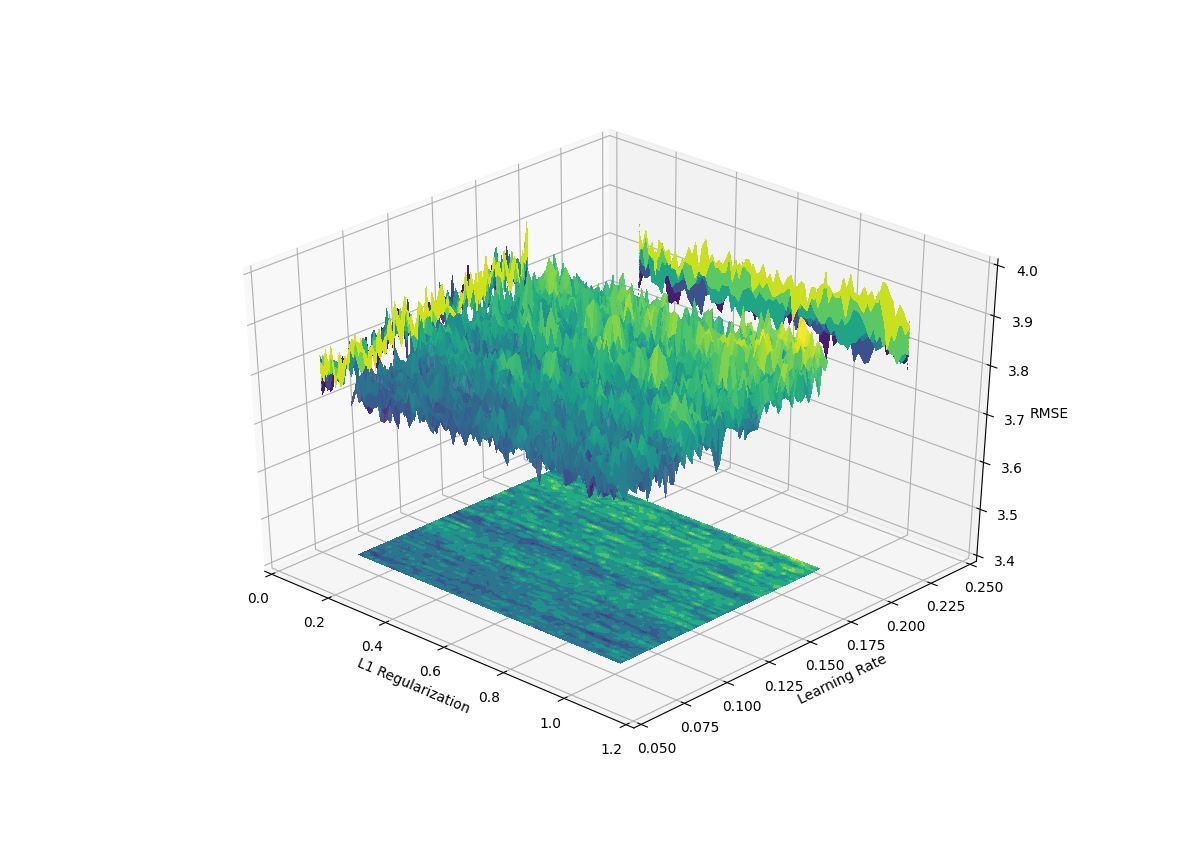
*Figure 7. Each panel shows the addition of sampled points. The samples are determined by the maximum of the aquisition function (green line).*

A More Realistic Example

In real world applications, the function we are trying to find the maximum of is never as smooth as what we previously used. Typically, the space of hyper-parameters or features of a model are noisy and sometimes lack overall structure. To demonstrate this we take take the Boston housing price dataset and conduct an extensive grid search of two hyperparameters (learning rate and l1 regularization) for a gradient boosted model (LightGBM). We plot the two parametes along with the average out of sample validiation metric (RMSE).

%matplotlib notebook
import numpy as np
import pandas as pd
import lightgbm as lgb

import matplotlib.pyplot as plt
from matplotlib import cm

from sklearn.datasets import load_boston
from sklearn.model_selection import GridSearchCV, KFold, train_test_split


# Load Boston Housing dataset
data = load_boston()
x_values = pd.DataFrame(data.data, columns=data.feature_names)
y_values = pd.Series(data.target)

n_steps = 80

x_train, x_test, y_train, y_test = train_test_split(
    x_values, y_values, test_size=0.2, random_state=42
)

fit_params = {
    'early_stopping_rounds': 500
}

grid_params = {
    'learning_rate': np.round(np.linspace(0.08, 0.2, n_steps), 4),
    'lambda_l1': np.round(np.linspace(0.1, 0.99, n_steps), 4)
}

kf = KFold(n_splits=5, shuffle=True, random_state=42)

clf = lgb.LGBMRegressor(
    n_estimators=5000,
    random_state=42
)

grid_search = GridSearchCV(
    clf,
    grid_params,
    scoring='neg_root_mean_squared_error',
    cv=kf,
    refit=True,
    verbose=0,
    n_jobs=8,
)

grid_search.fit(x_train, y_train, eval_set=[(x_test, y_test)], **fit_params)
grid_res = grid_search.cv_results_

mean_err = np.abs(grid_res['mean_test_score'])
param1 = grid_res['param_lambda_l1']
param2 = grid_res['param_learning_rate']
param1 = param1.compressed()
param1 = param1.astype(np.float)
param2 = param2.compressed()
param2 = param2.astype(np.float)

X = param1.reshape(n_steps, n_steps)
Y = param2.reshape(n_steps, n_steps)
Z = mean_err.reshape(n_steps, n_steps)

fig = plt.figure()
ax = fig.gca(projection='3d')
ax.plot_surface(
    X, Y, Z, rcount=500, ccount=500, alpha=0.9, cmap=cm.viridis, linewidth=0, antialiased=False
)

ax.set_xlabel('L1 Regularization')
ax.set_ylabel('Learning Rate')
ax.set_zlabel('RMSE')

cset = ax.contourf(X, Y, Z, zdir='z', offset=3.4, cmap=cm.viridis)
cset = ax.contourf(X, Y, Z, zdir='x', offset=0.0, cmap=cm.viridis)
cset = ax.contourf(X, Y, Z, zdir='y', offset=0.25, cmap=cm.viridis)

ax.set_xlim(0.0, 1.2)
ax.set_ylim(0.05, 0.25)
ax.set_zlim(3.4, 4.0)
plt.show()

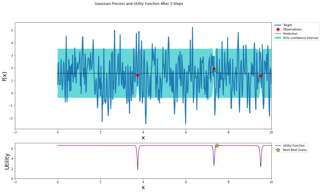
*Figure 8. 3D plot of the out of sample validation of the model (RMSE) versus the two hyper-pamaters of the model.*

To see how Bayesian optimization might perform in this type of environment we start with a noisy function \(f\left(x\right) = e^{sin\left(50x\right)} + sin\left(60e^{x}\right) + sin\left(70 sin\left(x\right)\right) + sin\left(x^{2}\right)\)

For this optimization I will use the Python package BayesianOptimization

from bayes_opt import BayesianOptimization
from bayes_opt import UtilityFunction
from matplotlib import gridspec

def posterior(optimizer, x_obs, y_obs, grid):
    optimizer._gp.fit(x_obs, y_obs)

    mu, sigma = optimizer._gp.predict(grid, return_std=True)
    return mu, sigma

def plot_gp(optimizer, x, y):
    '''
    source: https://github.com/fmfn/BayesianOptimization/blob/master/examples/visualization.ipynb
    '''
    fig = plt.figure(figsize=(16, 10))
    steps = len(optimizer.space)
    fig.suptitle(
        'Gaussian Process and Utility Function After {} Steps'.format(steps),
        fontdict={'size':30}
    )
    
    gs = gridspec.GridSpec(2, 1, height_ratios=[3, 1]) 
    axis = plt.subplot(gs[0])
    acq = plt.subplot(gs[1])
    
    x_obs = np.array([[res["params"]["x"]] for res in optimizer.res])
    y_obs = np.array([res["target"] for res in optimizer.res])
    
    mu, sigma = posterior(optimizer, x_obs, y_obs, x)
    axis.plot(x, y, linewidth=3, label='Target')
    axis.plot(x_obs.flatten(), y_obs, 'D', markersize=8, label=u'Observations', color='r')
    axis.plot(x, mu, '--', color='k', label='Prediction')

    axis.fill(np.concatenate([x, x[::-1]]), 
              np.concatenate([mu - 1.9600 * sigma, (mu + 1.9600 * sigma)[::-1]]),
        alpha=.6, fc='c', ec='None', label='95% confidence interval')
    
    axis.set_xlim((-2, 10))
    axis.set_ylim((None, None))
    axis.set_ylabel('f(x)', fontdict={'size':20})
    axis.set_xlabel('x', fontdict={'size':20})
    
    utility_function = UtilityFunction(kind="ucb", kappa=5, xi=0)
    utility = utility_function.utility(x, optimizer._gp, 0)
    acq.plot(x, utility, label='Utility Function', color='purple')
    acq.plot(x[np.argmax(utility)], np.max(utility), '*', markersize=15, 
             label=u'Next Best Guess', markerfacecolor='gold', markeredgecolor='k', markeredgewidth=1)
    acq.set_xlim((-2, 10))
    acq.set_ylim((0, np.max(utility) + 0.5))
    acq.set_ylabel('Utility', fontdict={'size':20})
    acq.set_xlabel('x', fontdict={'size':20})
    
    axis.legend(loc=2, bbox_to_anchor=(1.01, 1), borderaxespad=0.)
    acq.legend(loc=2, bbox_to_anchor=(1.01, 1), borderaxespad=0.)

# ---------------------------------------------------------
# This is the actual function that we would like to predict
# ---------------------------------------------------------
f = lambda x: np.exp(np.sin(50*x)) + np.sin(60*np.exp(x)) + np.sin(70*np.sin(x)) + np.sin(np.power(x, 2))
x = np.atleast_2d(np.linspace(0, 10, 500)).T
y = f(x)

optimizer = BayesianOptimization(
    f, 
    pbounds={'x': (0, 10)},
    random_state=42,
    verbose=0
)

optimizer.maximize(init_points=3, n_iter=0, kappa=3)

plot_gp(optimizer, x, y)

optimizer.maximize(init_points=0, n_iter=100, kappa=3)
plot_gp(optimizer, x, y)

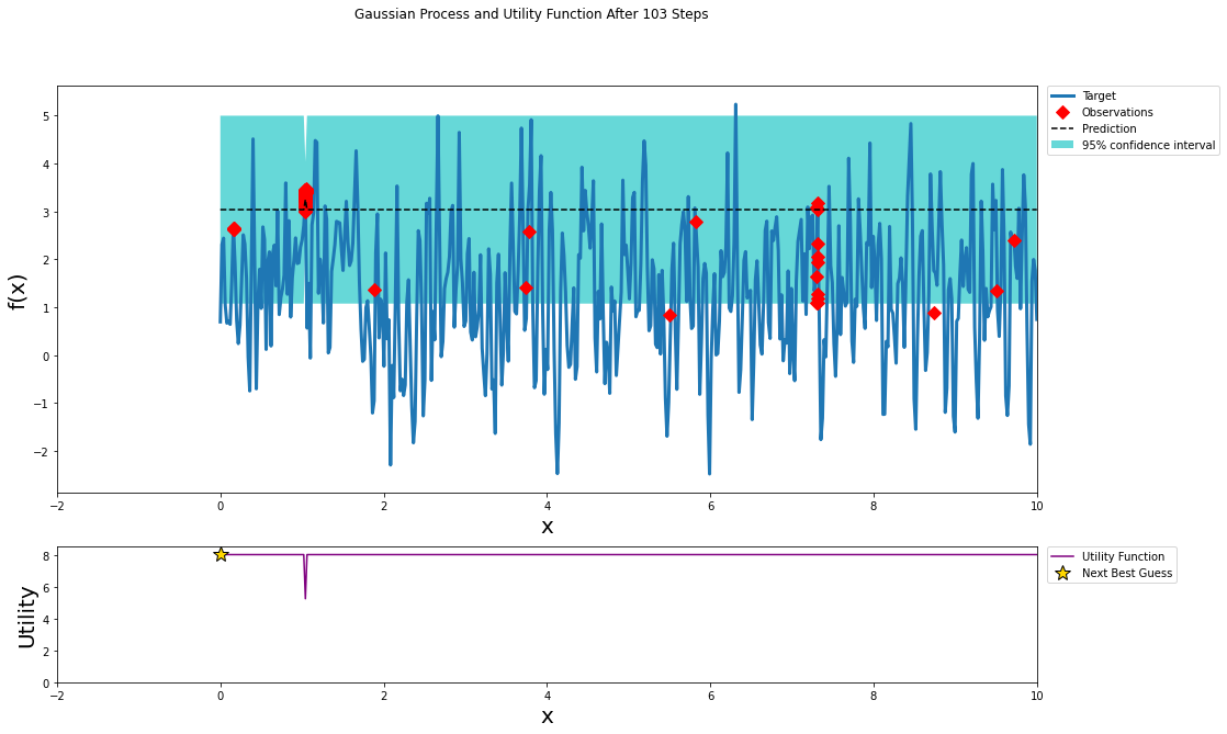
The function we specified was periodic in nature and periodic kernel may have provided a better fit; however, when optimizing hyper-parameters you can not guarantee that the model performance within the hyper-parameter space is periodic.

For noisy functions such as the one shown above and space of hyper-parameters that we previously explored there are many local maximums. These sharp peaks make it difficult to find the global max. Bayesian optimization does a decent job of exploring local maximums. In the pursuit of the global maximum Bayesian optimization may not be better than a random grid search.

A significant disadvantage of Bayesian optimization is the inability to handle discrete or categorical variables in a fundamental way. You can coerce the output of Bayesian optimization to be an integer; however, the algorithm is optimizing on the assumption that the variable is continuous. In addition, for Bayesian Optimization, categorical variables must be encoded such that they have implied ordinality.

The code provided below tunes hyper-parameters for the Boston housing data using both random grid search and Bayesian optimization. Originally, I was going to use that code to show that random grid search performs just as well as Bayesian optimization; however, a better solution was found with Bayesian optimization. This came at the cost of computation time. There is an additional cost in calculating the Gaussian model as well as finding the maximum of the acquisition function. In addition, Bayesian Optimization is not easily parallelized. This type of optimization is very sequential. There is research on how to make Bayesian optimization run in a parallel fashion.

Conclusions

There is no perfect model or approach in data science. Each methodology has its advantages and disadvantages. Make you understand what these are and that will help you determine the best approach for your application.

References

Franceschi, L., Donini, M., Frasconi, P. and Pontil, M., 2017, August. Forward and reverse gradient-based hyperparameter optimization. In Proceedings of the 34th International Conference on Machine Learning-Volume 70 (pp. 1165-1173). JMLR. org.

Görtler, et al., “A Visual Exploration of Gaussian Processes”, Distill, 2019.

Maclaurin, D., Duvenaud, D. and Adams, R., 2015, June. Gradient-based hyperparameter optimization through reversible learning. In International Conference on Machine Learning (pp. 2113-2122).

Murphy, K.P., 2012. Machine learning: a probabilistic perspective. MIT press.

Other Learning Resources

from sklearn.model_selection import RandomizedSearchCV
import numpy as np
import pandas as pd
import lightgbm as lgb

import matplotlib.pyplot as plt
from matplotlib import cm

from sklearn.datasets import load_boston
from sklearn.model_selection import GridSearchCV, KFold, train_test_split, cross_val_score

from bayes_opt import BayesianOptimization


data = load_boston()
x_values = pd.DataFrame(data.data, columns=data.feature_names)
y_values = pd.Series(data.target)

n_steps = 200
n_iters = 500

x_train, x_test, y_train, y_test = train_test_split(
    x_values, y_values, test_size=0.2, random_state=42
)

fit_params = {
    'early_stopping_rounds': 50,
    'verbose': 0,
}

grid_params = {
    'learning_rate': np.linspace(0.08, 0.2, n_steps),
    'lambda_l1': np.linspace(0.1, 0.99, n_steps),
    'feature_fraction': np.linspace(0.1, 0.99, n_steps),
}

clf = lgb.LGBMRegressor(
    n_estimators=5000,
    random_state=42
)
kf = KFold(n_splits=5, shuffle=True, random_state=42)

# ------------------
# Random Grid Search
# ------------------
grid_search = RandomizedSearchCV(
    clf,
    grid_params,
    scoring='neg_root_mean_squared_error',
    cv=kf,
    n_iter=20,
    refit=True,
    verbose=0,
    random_state=42,
    n_jobs=8,
)

grid_search.fit(x_train, y_train, eval_set=[(x_test, y_test)], **fit_params)
grid_res = grid_search.cv_results_
mean_score = np.abs(grid_res['mean_test_score'])
min_rnd_search = np.minimum.accumulate(mean_score)
n_trails = np.arange(1, n_iters+1)

# ---------------------
# Bayesian Optimization
# ---------------------
def optimize_lgbm(x, y):
    def lgbm_cv(learning_rate, lambda_l1, feature_fraction):

        params = {
            'objective': 'regression',
            # 'n_estimators': 5000,
            'learning_rate': learning_rate,
            'lambda_l1': lambda_l1,
            'feature_fraction': feature_fraction,
            'random_state': 42
        }

        lgb_dataset = lgb.Dataset(x, y)

        cv_results = lgb.cv(
            params,
            lgb_dataset,
            num_boost_round=5000,
            folds=kf,
            # nfold=5,
            early_stopping_rounds=50,
            metrics='rmse',
            stratified=False,
        )

        return -cv_results['rmse-mean'][-1]

    optimizer = BayesianOptimization(
        f=lgbm_cv,
        pbounds={
            "learning_rate": (0.08, 0.2),
            "lambda_l1": (0.1, 0.99),
            "feature_fraction": (0.1, 0.99)
        },
        random_state=42,
        verbose=-1
    )
    optimizer.maximize(n_iter=n_iters)
    return optimizer

opt = optimize_lgbm(x_values, y_values)