Introduction
Where is the intersection of social-economic behavior and mathematics? Is it possible to use fundamental equations to model population behavior? A while back a colleague, Kevin James, and I created an interactive report detailing a hypothetical forced migration scenario in Yemen. That report gave a high-level graphic overview of the project as well as allowed the user to explore possible scenarios. In this short blog post, we explore some of the technical aspects of the modeling. Even though statistical modeling is all the hotness right now, there are still applications that work well with modeling physical principals. For this project, I attempted to modeled human behavior (migration) using a fundamental law of physics, heat conduction (the heat equation).
Before we dive in, I would like to highlight the work of Paul Millhouser, a geospatial ecologist, who modeled the migration of Colorado wildlife using the idea of electrical conductivity.
This project was a proof of concept. The code used in creating the thermal resistance layers and numerically solving the transient and steady state heat equations is located in this repository. Be forewarned that I have not put in the effort to clean up the code (as I should have) before making public.
Purpose
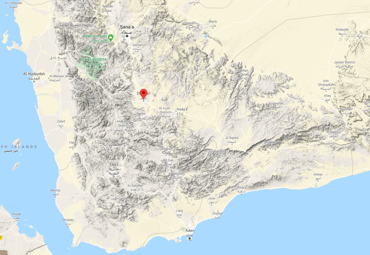
The idea behind this project was to develop a method to help aid organizations better understand what factors influence migration paths so that they can potentially respond with aid more effectively. We choose Dhamar, Yemen as the epicenter for the forced migration event for several reasons. Yemen is one of the Middle East’s poorest countries and has been embroiled in a complex power play strife with conflict and corruption. Beginning in the 1990s, the Houthi movement emerged as an opposition to the former Yemeni president Ali Abdullah Saleh. The Houthis charged Saleh with massive financial corruption and criticized him for being backed by Saudi Arabia and the United States. During the popular uprising in 2011, president Ali Abdullah Saleh, who had been in rule for 33 years was forced out of his position and was replaced by his deputy, Abd Rabbu Mansour Hadi. After this transition, with the support of external countries, efforts were made to broker peace between the various factions in Yemen through the National Dialogue Conference. Although the Houthis took part in this conference they later rejected the deal. In 2014, in a somewhat ironic move, the Houthis forged an alliance with the former President Saleh and took over the government in Sanaa, replacing the government lead by Hadi. This was the start of a full-blown conflict. A coalition lead by Saudi Arabia and the United Arab Emirates (UAE) launched an aerial bombing campaign against Huthis forces in 2015 marking the beginning of a full-blown armed conflict between the Huthis and coalition-backed armed groups.
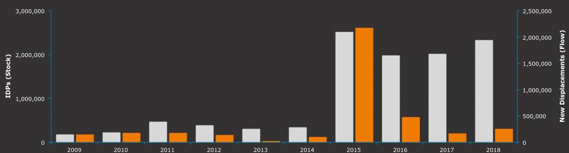
The conflict in Yemen has caused what the United Nations labels as the world’s worst humanitarian crisis. The Yemen population is constantly displaced as families flee and return with the ebb and flow of armed conflict in the country. Many families have been forced to return to their homes near the front lines of violent conflicts because of the cost associated with displacement. Below is a figure from the Internal Displacement Monitoring Centre (IDMC) showing the annual conflict and disaster displacement figures for Yemen.
The city of Dhamar in Yemen was chosen as the epicenter for the forced migration event, not because of any particular current political situation but because of the diversity of landscape and social-economic conditions surrounding the city. Dhamar is situated on the main road that connects Sana’a, Yemen’s largest city, with a number of other governorates.
Methodology
The main premise I took for modeling migration was to assume that a population under duress would take a path of least resistance to flee a conflict area. With this idea in mind, we can simulate migration using the parabolic differential equation (heat equation) with variable thermal conductivity. The equation looks like:
\[\frac{U}{\partial t} = \nabla \cdot \left(\alpha \nabla U \right)\]Where \(U\) is the temperature at any point \((x,y)\) and any time \(t\), and \(\alpha\) is the thermal diffusivity. The diffusivity is the rate at which heat can spread through a medium and is related to the inverse of thermal resistivity. How the heat flows, or the heat flux, represents the flow of population from the epicenter. Theoretically, in a life or death scenario, people will move along the path of least resistance. The resistance function describes how the population moves about the terrain. The resistance function acts as the link between human behavior and mathematical modeling.
Thermal Resistance
There are many different factors that can influence how a person travels over a geographic area. These factors can be physical like the slope of the terrain, they can be situational like an outbreak of armed conflict, or they can be economic-based. There are two main challenges in finding the resistance to travel over a geographic area:
- Finding the right factors which impact a populations desire to travel in certain regions
- Quantifying these factors into actual resistance to travel
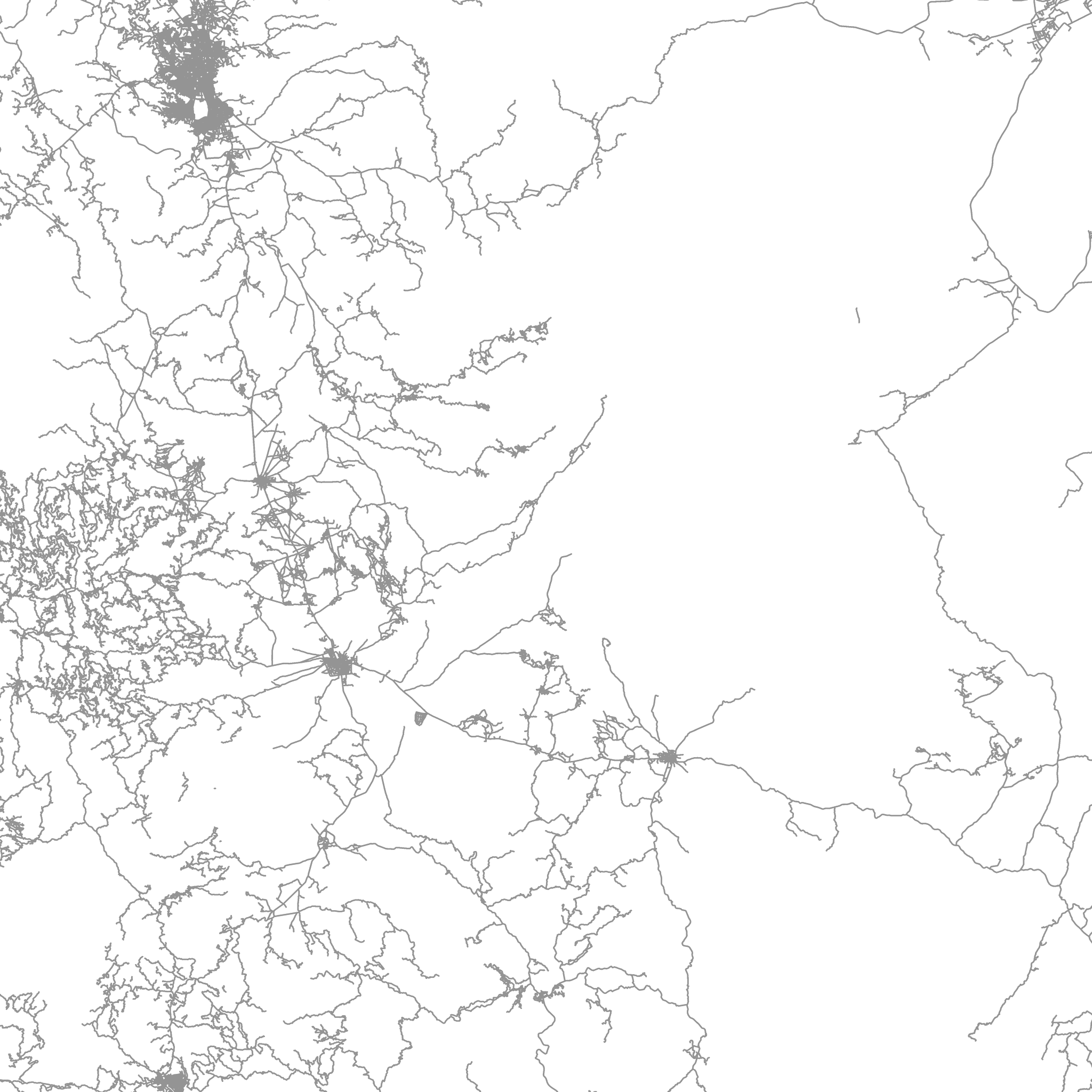
For this proof of concept, I went with four different types of layers of resistance. The first layer is roads and waterways. The thought is that roads are favorable to travel along. They offer a paved surface, typically of low slope, in which a person can travel along. However, roads are also a pathway to move armed soldiers between conflicts. This type of traffic would cause migrating populations to avoid travel along roads. For this proof of concept, we did not consider this situational event and set all roads as favorable. In addition, we set the waterways as unfavorable to travel across. The road and water way data is derived from Open Street Maps.
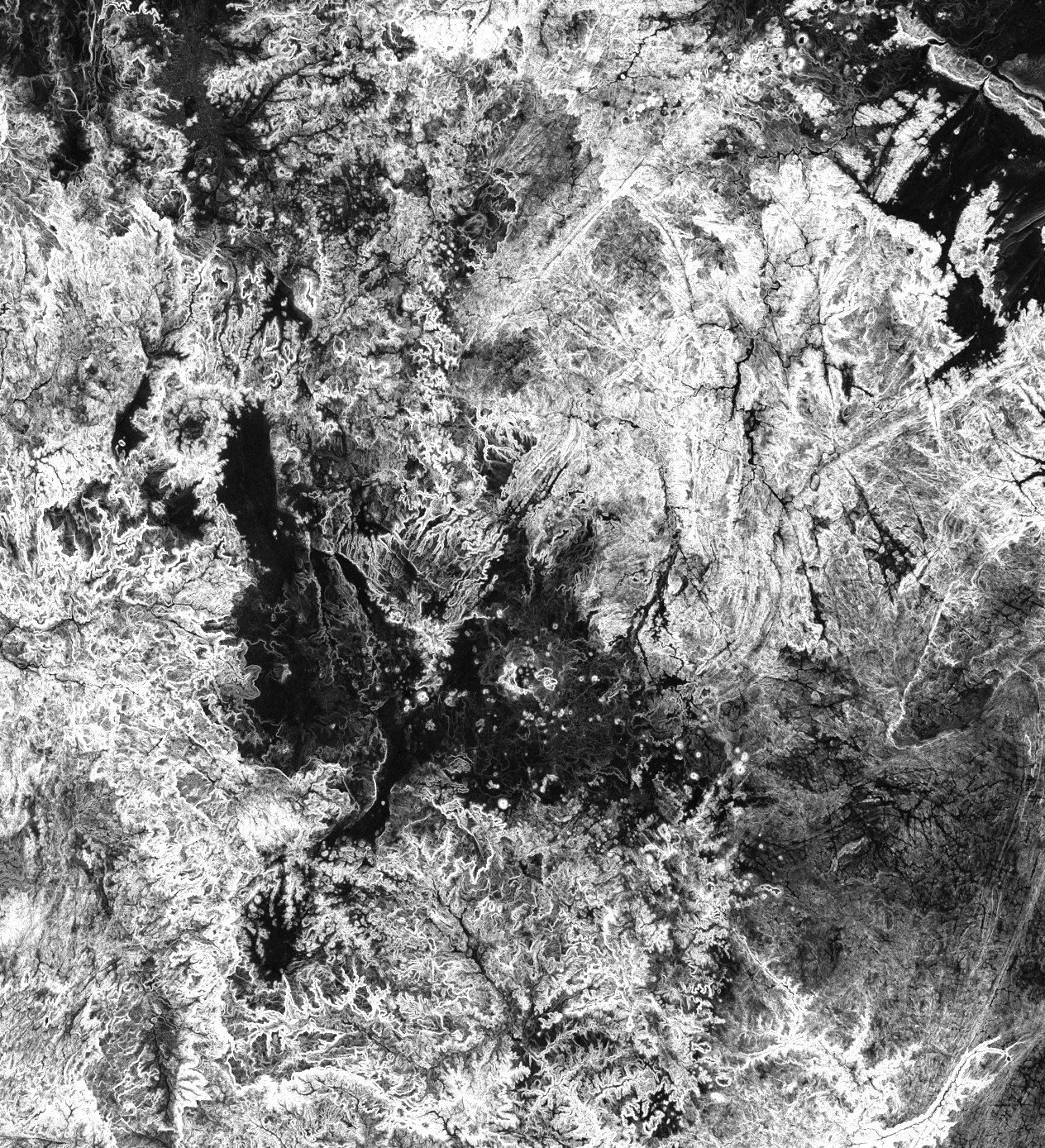
The second layer is the slope of the terrain. Steep slopes are harder to travel across than flat ground, so migrants may plan their paths to avoid steep terrain. As it turns out there are actually mathematical functions to calculate travel time based on the slope of the terrain (Campbell et al, 2019) which are fit from empirical data. Based on previous research I decided to use an exponential relationship between travel resistance and slope of the terrain. Data to calculate slope comes from the Japan Aerospace Exploration Agency (JAXA) Digital Elevation Model at a 30 meter resolution.
The third layer I used was the administrative boundaries for Yemeni districts or Modeeriyyah. A population may choose to avoid traveling across administrative boundaries due to road blocks, security checks, or regional differences in politics and religion. Similar to most administrative boundaries, there is no physical analog to these boundaries. I suspect that when a population migrates they do not really consider an imaginary boundary. I don’t think I would include this layer in future iterations of this project.
The final layer is the United Nations Humanitarian Needs Overview inter-sector needs severity index. The needs severity index is a seven-point scale (0 to 6), with higher numbers indicating greater need. This index is based on considerations such as population health, water, sanitation, and hygiene, nutrition, shelter, education, and food and physical security.
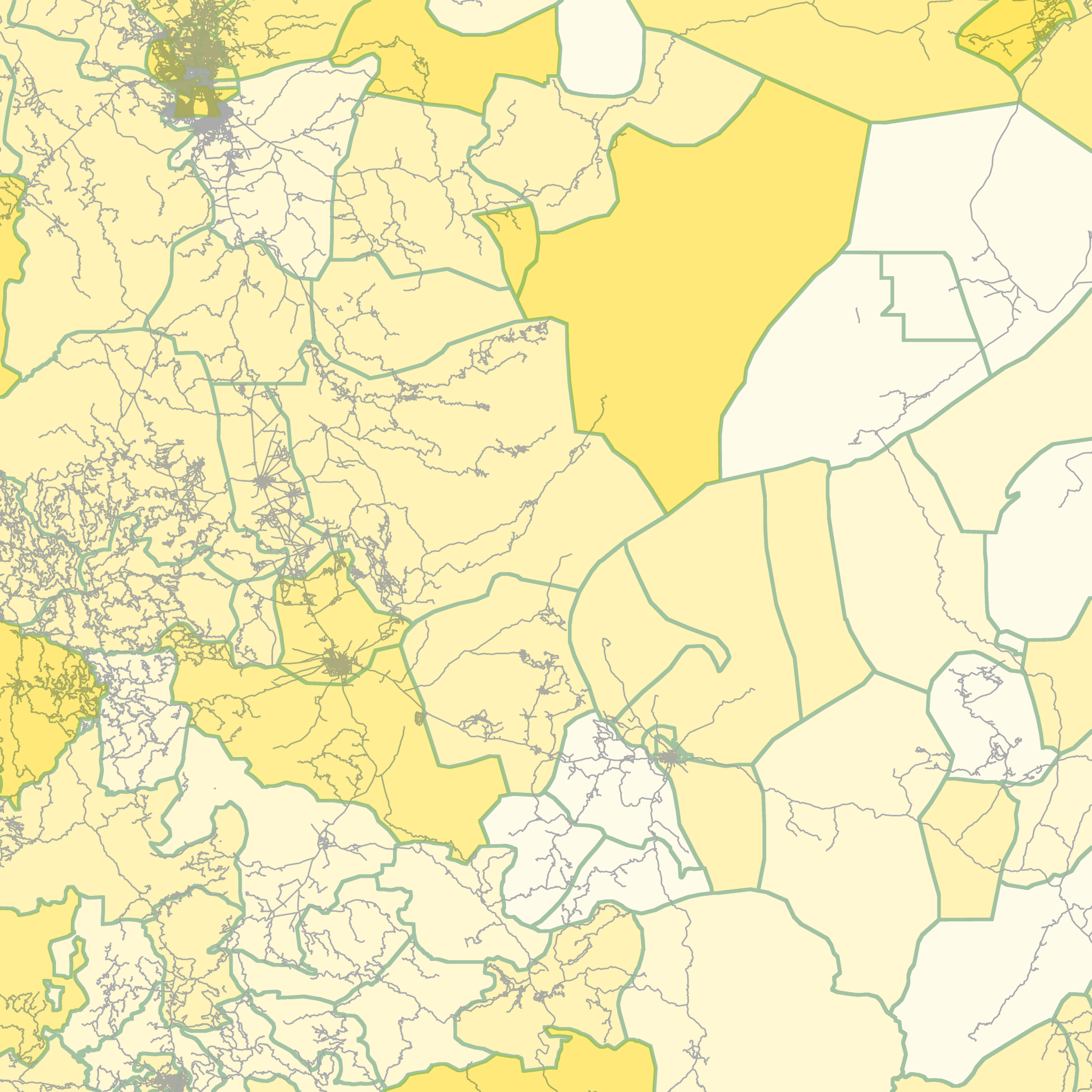
These layers are added together into a single thermal resistance layer. What type of factors are included in the resistance and how these factors are weighted is where I believe the intersection of human behavior and mathematical modeling exists. I think there are some universal factors which will influence how people migrate over distances; however, there are also local cultural factors which can impact the movement. In addition, the influence of various factors on travel resistance greatly depends on the characteristics of the affected population. How desperate is the population to move from the epicenter?
Although for this proof of concept, I did not incorporate local knowledge of the population, I think this should be done in future modeling efforts.
Now that we have a version of our thermal resistivity that corresponds to how we think a population will travel, it’s time to set up the heat equation.
Heat Equation
The likelihood that migrating individuals take a particular path will be represented by the heat flux along that path. This is strictly not a probability because the sum of the heat flux over the surface is not equal to one. Since the heat flux is calculated from the temperature field, this calculation occurs in two steps. First we calculate the temperature field. Then from the temperature field we calculate the heat flux. We start with the most basic form of the heat equation.
\[\frac{U}{\partial t} = \nabla \cdot \left(\alpha \nabla U \right)\]You may have come across this equation in partial differential equations class on in a physics class. Typically, for these pedagogical excercises one assumes that the thermal diffusivity is constant. This simplifies the equation by allowing the gradient to pass and become the Laplace operator on \(U\). In our case the thermal diffusivity (inverse of the resistance) is a function of both \(x\) and \(y\) coordinates. We have to take care when taking the partial derivative of the thermal diffusivity. After expanding out terms we have.
\[\frac{U}{\partial t} = \alpha \left(\frac{\partial^{2}U}{\partial x^{2}} + \frac{\partial^{2}U}{\partial y^{2}} \right) + \frac{\partial \alpha}{\partial x}\frac{\partial U}{\partial x} + \frac{\partial \alpha}{\partial y}\frac{\partial U}{\partial y}\]At this point we can go two different ways for solving this equation. We can solve the steady state version of this where we ignore the time component.
\[\frac{U}{\partial t} = 0\]Or we can solve the transient version of the case where we consider the partial derivative with respect to time. For this project we looked at both the steady state and the transient solution. The thought was that the steady state shows the likelihood of travel over the course of the entire migratory event while the transient solution shows the evolution of migration through time.
Before we jump into the solutions for steady state and transient, a note on the boundary conditions. Dirichlet boundary conditions were applied to the edges of the map, setting the temperatures to zero. A constant circular source temperature was used at the epicenter of the migratory event.
Steady State Solution
For solving the steady state problem I used a central difference of order \(O\left(h^{4}\right)\) to approximate the first and second derivatives. In particular,
\[f'\left(x_{0}\right) \approx \frac{-f_{2}+8f_{1}-8f_{-1}+f_{-2}}{12h}\] \[f''\left(x_{0}\right) \approx \frac{-f_{2}+16f_{1}-30f_{0}+16f_{-1}+f_{-2}}{12h^{2}}\]Once the center difference approximations are substituted in for the first and second derivatives the temperature at point \(i,j\) can be written in terms of its thermal diffusivity and neighboring temperature and thermal diffusivity. A coefficient matrix of the terms for each of the temperatures at point \(i,j\) can be set up. This leaves us with a linear system of equations for which we can solve taking the inverse of the coefficient matrix.
Transient Solution
We must take care to ensure numerical stability when solving for the transient case. I chose to use the Runge-Kutta-Fehlburg (RK45) method which allows for adaptive step size. This embedded method adapts the step size to control the errors and ensure stability of the algorithm. Errors are estimated by comparing two different approximations to the solution. The first is of the order \(O(h^{4})\) and the second is of the order \(O(h^{5})\).
Heat Flux
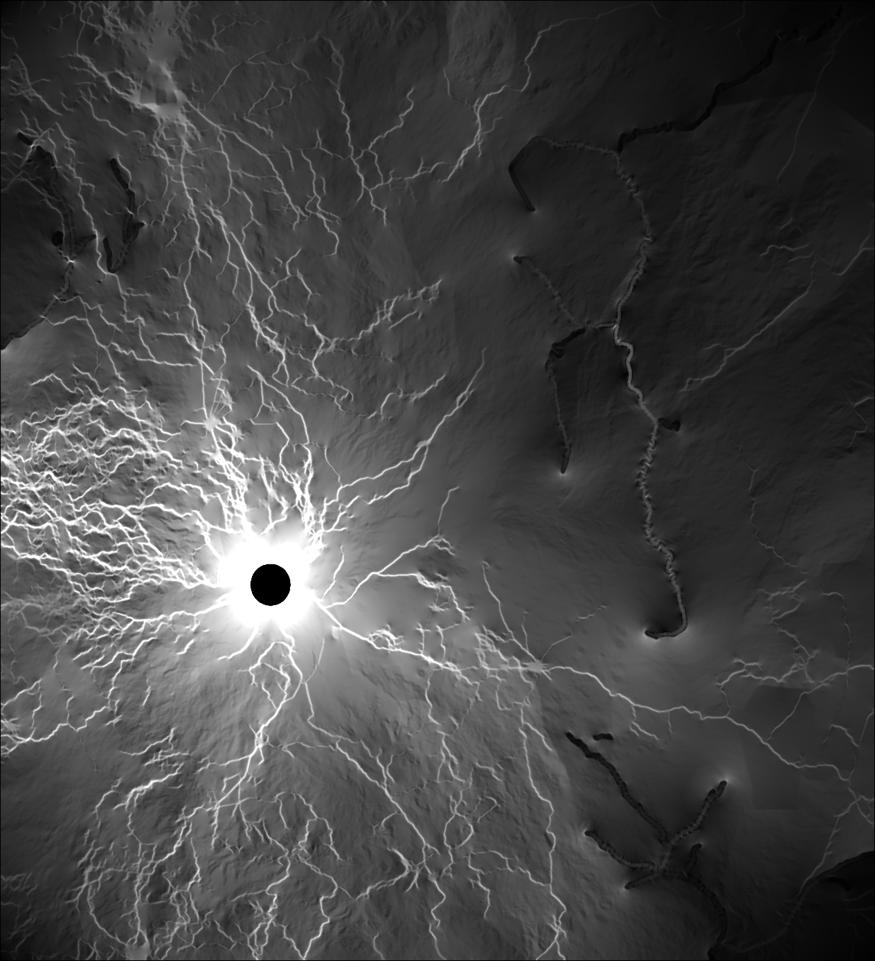
Once the temperature fields are calculated the heat flux can be derived using the equations,
\[\phi_{q} = -k \nabla T\]We approximate the derivatives with a central difference formulation of order \(O(h^{2})\). The figures below show both the solutions for the steady state heat flux and and the transient heat flux

Conclusions
Using the concept of resistance layers we attempt to quantify human decisions in terms of migratory behavior. With a thermal resistance layer we use the heat equation to find the heat flux across a geographic region. Significant amount of work remains in determining the most appropriate factors to include in the resistance layers as well as determining their relative importance. Please feel free to take all or part of this work to adapt to your own project. If you see any errors or would like to discuss, feel free to reach out to me through the email button below.