Introduction
For every model prediction we make there is an underlying uncertainty in that prediction. One of the key aspects of operationalizing AI models, is to understand the uncertainties of the predictions. If you are going to make a decision or take an action based on a model that could impact the operation of a multimillion dollar piece of equipment it’s best to clearly understand the uncertainties in that prediction. In this post, we explore two categories of model uncertainty and illustrate these uncertainties through practical examples. Note that this post heavily draws upon Guilherme Duarte Marmerola’s excellent post.
Aleatoric vs Epistemic Uncertainty
Model uncertainty can be broken down into two different categories, aleatoric and epistemic. These are often referred to as risk (aleatoric uncertainty) and uncertainty (epistemic uncertainty). Because the term “uncertainty” can refer to a specific type of uncertainty (epistemic) or the overall uncertainty of the model, I will use the terms aleatoric and epistemic in this blog post.
At a high level, epistemic uncertainties are uncertainties that can be reduced by gathering more data or refining the models, while aleatoric uncertainties can not be reduced. Aleatoric uncertainty is intrinsic in the randomness of the process we are trying to model. Say for example, we wanted to predict the performance of a compressor pump based on its operating conditions. Each compressor is slightly different. There may be small differences in the tolerances of manufactured pieces or how the pumps were assembled. These slight differences will lead to different efficiencies under similar operating conditions. Although we can work to quantify what the aleatoric uncertainty is, on the modeling and data side, we can not reduce it.
Epistemic uncertainty on the other hand can be addressed by collecting more data or building better models. Say we have a new piece of equipment for manufacturing and we would like to predict the efficiency of that equipment. Since we have such a limited set of historic data for the equipment the models will start out with a relatively high level of epistemic uncertainty. As we collect more data we will reduce the epistemic uncertainty.
Uncertainty Through Data
So what does aleatoric and epistemic uncertainty look like in data. We start by generating data based on the equation,
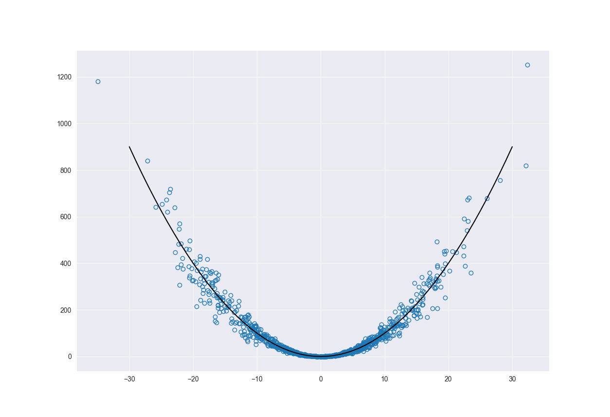
\[y = x^{2} + \epsilon\]We sample the \(x\) values from a normal distribution with a mean zero and standard deviation of 0.1, \(N(0, 0.01)\). This has the effect of making the majority of our observations cluster around zero. As we move further away from zero on the positive and negative sides we have fewer and fewer observations. The \(\epsilon\) part of the equation adds noise to the original function (\(x^{2}\)). The noise is normally distributed; however, the standard deviation is a function of \(x\) and changes as \(0.1 + 0.2*x^{2}\). This has the effect of changing the magnitude of the noise that gets added to the original signal. As one moves further away from zero, the noise increases. This is called heteroscedastic noise because the variance of the noise changes along the x-axis. We could have added a constant variance noise to the signal; however, the variability will help show the change in our models uncertainty.
The figure below shows the main function (black line) along with the function sampled according to \(N(0, 0.01)\) with added heteroscedastic noise.
import numpy as np
import matplotlib.pyplot as plt


# Sample x values
x = np.random.normal(0, 0.1, 1000) * 100
x2 = np.arange(-30, 31, 1)

# Heterscodastic noise
eps = np.random.normal(scale=(0.1 + 0.2*np.power(x, 2)))

# Actual function to predict
y = np.power(x, 2) + eps
y2 = np.power(x2, 2)

fig, ax = plt.subplots()
ax.plot(x, y, 'o', fillstyle='none')
ax.plot(x2, y2, 'k-')
ax.grid(True)
plt.show()
We added noise and sampled \(x\) from a distribution to illustrate both aleatoric and epistemic uncertainty. The heteroscedastic noise represents variability of our system and therefore the aleatoric uncertainty. It’s something that we can not reduce. As the noise increases away from 0 so does our epistemic uncertainty.
The way we sampled the \(x\) values represents the epistemic uncertainty. This uncertainty will also increase as we move away from the origin. The reason for this is because we have less data points to train the model on the further out we go. This is a reducible error as we could go out and collect more data points, given enough time and resources.
We can start by training and testing a model to fit the data. We build a very simple neural network to fit the data.
from keras import backend as K
from keras.models import Model
from keras.callbacks import EarlyStopping
from keras.layers import Input, Dense


def build_model():
    inputs = Input(shape=(1,))
    model = Dense(32, activation='relu')(inputs)
    model = Dense(16, activation='relu')(model)
    output = Dense(1, activation='linear')(model)
    simple_model = Model(inputs, output)
    return simple_model


simple_model = build_model()
simple_model.compile(optimizer='adam', loss='mean_absolute_error')

earlystop = EarlyStopping(monitor='val_loss', patience=10)

model_hist = simple_model.fit(
    x, y,
    batch_size=64,
    epochs=700,
    callbacks=[earlystop],
    shuffle=True,
    validation_split=0.2
)

x_pred = np.arange(-30, 31, 1)
x_pred = x_pred.reshape(x_pred.shape[0], -1)
pred = simple_model.predict(x_pred)

fig, ax = plt.subplots()
ax.plot(x, y, 'o', fillstyle='none')
ax.plot(x_pred, pred, '-')
ax.grid(True)
plt.show()

Now that we have a dataset that represents both aleatoric and epistemic uncertainty as well as a model to estimate our underlying function, let’s dig into how we can quantify the uncertainty of the model prediction.
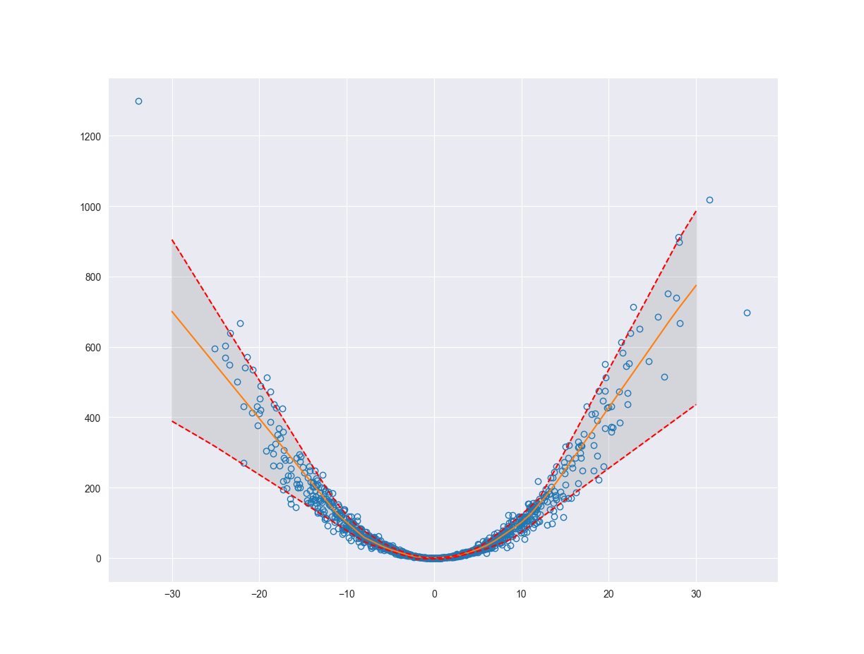
Aleatoric Uncertainty
We can estimate the variability of our system (aleatoric uncertainty) using something called quantile regression. The idea behind quantile regression is that we fit a function or line which splits the data into the \(Nth\) quantile and the rest of the data. So the \(Nth\) quantile of data would fall above or below the line and the rest of the data would fall on the opposite side. This will help us quantify the variability of the system by finding the boundaries for the outliers of our function, where outliers are defined according to the quantile that we choose. Below we will fit a model to the \(10th\) and \(90th\) quantiles. This will give us an upper and lower bound estimating the aleatoric uncertainty of the system.
So how does one accomplish quantile regression with a neural network or gradient boosted model. Koenker and Hallock, 2001 generalize the idea of minimizing the sum asymmetrically weighted absolute residuals to yield quantiles. One can obtain an estimate of any quantile by tilting the \(l1\) loss function by an appropriate amount. This is known as tilted loss or pinball loss. The function looks like,
\[L_{\tau}(y-y^{*}) = \begin{cases} \tau(y-y^{*}),& \text{if } y\geq y^{*}\\ -(1-\tau)(y-y^{*}), & \text{if } y \lt y^{*} \end{cases}\]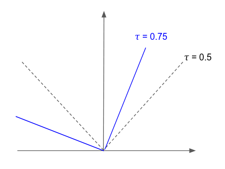
Notice that if the tilting parameter is \(\frac{1}{2}\) or \(50th\) quantile we recover the \(l1\) loss function.
def pinball_loss(q):
    def loss(y_actual, y_pred):
        return K.mean(K.maximum(q*(y_actual-y_pred), (q-1)*(y_actual-y_pred)), axis=1)
    return loss


# 10th quantile
simple_model_q10 = build_model()
simple_model_q10.compile(optimizer='adam', loss=pinball_loss(0.10))

earlystop = EarlyStopping(monitor='val_loss', patience=10)

model_hist = simple_model_q10.fit(
    x, y,
    batch_size=64,
    epochs=700,
    callbacks=[earlystop],
    shuffle=True,
    validation_split=0.2
)

pred_q10 = simple_model_q10.predict(x_pred)
delq10 = pred.flatten() - pred_q10.flatten()

# 90th quantile
simple_model_q90 = build_model()
simple_model_q90.compile(optimizer='adam', loss=pinball_loss(0.90))

earlystop = EarlyStopping(monitor='val_loss', patience=10)

model_hist = simple_model_q90.fit(
    x, y,
    batch_size=64,
    epochs=700,
    callbacks=[earlystop],
    shuffle=True,
    validation_split=0.2
)

pred_q90 = simple_model_q90.predict(x_pred)
delq90 = pred_q90.flattnen() - pred.flatten()

fig, ax = plt.subplots()
ax.plot(x, y, 'o', fillstyle='none')
ax.plot(x_pred, pred, '-')
ax.plot(x_pred, pred_q90, 'r--')
ax.plot(x_pred, pred_q10, 'r--')
ax.fill_between(x_pred.flatten(), pred_q10.flatten(), pred_q90.flatten(), color='grey', alpha=0.2)
ax.grid(True)
plt.show()
Before we start talking about the practical applications let’s take a look at how we can quantify the epistemic uncertainty.
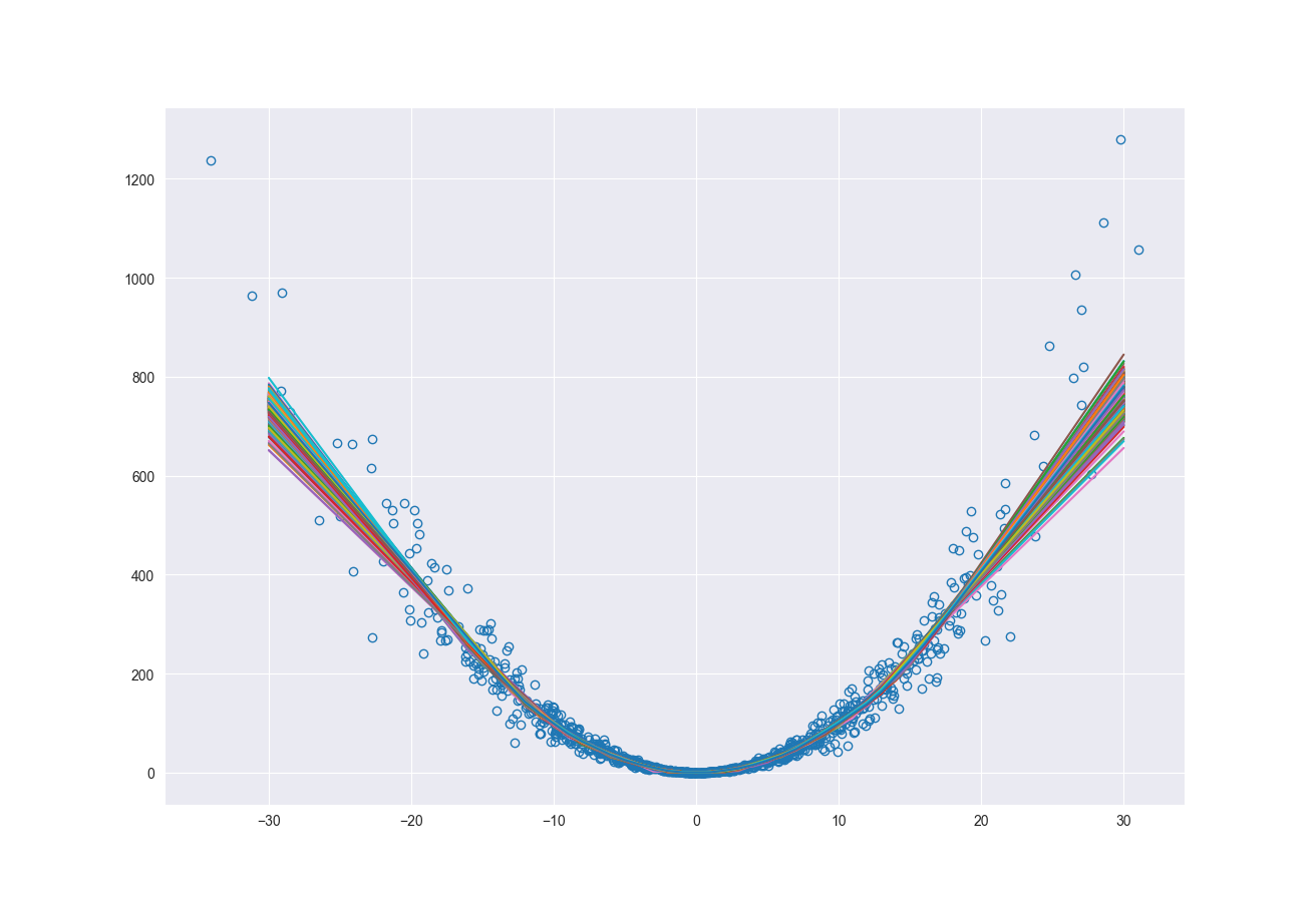
Epistemic Uncertainty
One of the many ways to estimate epistemic uncertainty in a model is to use bootstrapping to resample the original data set and re-train the model. This is a relatively simple method; however, it is computationally expensive. Every time you resample you must retrain the model. The more the number of resamplings, the better the estimate of the uncertainty. There are other methods for finding the epistemic uncertainty such as Monte Carlo Dropout (Gal and Ghahramani, 2016) and randomized prior functions (Osband, Aslanides, and Cassierer, 2018). Under sufficient conditions, resampling the original dataset is a reasonable representation of natural variance of the dataset. So, how does this capture epistemic uncertainty? If you consider our original synthetic data set the density of data points decreases as we move away from zero. As we resample and retrain the model, the areas with lower density of data points will see larger changes in model fit. Resampling at the low densities can cause the relationship between the independent and dependent variables to look very different.
Programmatically, as shown below, we resample \(N\) times, retrain the model and make predictions with each of those new models. Now for each point we have a distribution of possible prediction values. The minimum and maximum across those distributions represent the lower and upper bounds of our epistemic uncertainty.
from sklearn.utils import resample

n_iters = 500
n_sample_size = int(x.shape[0] * 0.6)
preds = []
earlystop = EarlyStopping(monitor='val_loss', patience=10)

for i in range(n_iters):
    x_boot, y_boot = resample(x, y, n_samples=n_sample_size)
    simple_model = build_model()
    simple_model.compile(optimizer='adam', loss='mean_absolute_error')

    model_hist = simple_model.fit(
        x, y,
        batch_size=64,
        epochs=700,
        callbacks=[earlystop],
        shuffle=True,
        validation_split=0.2,
        verbose=0
    )

    preds.append(simple_model.predict(x_pred).flatten().tolist())

    print(f"Finished model for iteration: {i}")

preds = np.asarray(preds)
upper_bnd = np.max(preds, axis=0)
delupper = upper_bnd - pred.flatten()
lower_bnd = np.min(preds, axis=0)
dellower = pred.flatten() - lower_bnd

fig, ax = plt.subplots()
ax.plot(x, y, 'o', fillstyle='none')
ax.plot(x_pred, pred, '-')
ax.plot(x_pred, upper_bnd, 'r--')
ax.plot(x_pred, lower_bnd, 'r--')
ax.fill_between(x_pred.flatten(), lower_bnd, upper_bnd, color='grey', alpha=0.2)
ax.grid(True)
plt.show()

Consolidating Uncertainty
Now that we have estimates for our epistemic and aleatoric uncertainty we can aggregate these together to determine our overall model uncertainty. These uncertainties should be independent and therefore we can add them in quadrature.
\[uncertainty_{total} = \sqrt{(aleatoric)^{2} + (epistemic)^{2}}\]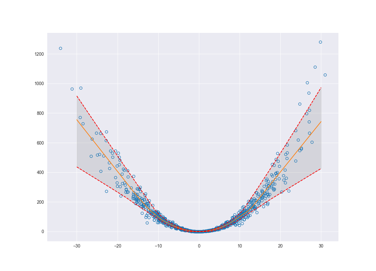
Applications
Practically, how would one use these uncertainty intervals? There are several ways you can view the bounds. Say you have a model that predicts the yield or efficiency of a certain process based on the operational parameters of that process. If the uncertainty of the predictions are consistently outside the bounds of acceptable yields, it is a good indication that the model should not be operationalized. At that point you should go back and re-evaluate the data and models.
Another way to view the uncertainty bounds is in terms of anomaly detection. If we have a prediction as well as well defined uncertainty bounds, we can compare this to the actual observed value. It is reasonable to classify actual values that fall outside of the uncertainty bounds as anomalies.
References
Gal, Y. and Ghahramani, Z., 2016, June. Dropout as a bayesian approximation: Representing model uncertainty in deep learning. In international conference on machine learning (pp. 1050-1059).
Koenker, R. and Hallock, K.F., 2001. Quantile regression. Journal of economic perspectives, 15(4), pp.143-156.
Osband, I., Aslanides, J. and Cassirer, A., 2018. Randomized prior functions for deep reinforcement learning. In Advances in Neural Information Processing Systems (pp. 8617-8629).