Introduction
This is a cautionary tale of using Dynamic Time Warping (DTW). We often see examples of successful applications of algorithms and models; however, this is an example when things do not go according to plan. Although we all enjoy talking about our success, I think we should take more time to discuss things we tried and didn’t work. Maybe others can provide insight on how to make our failed task work or we can help them avoid a similar stumble.
I was working with a physical industrial system that had multiple measurements throughout the process. The main goal was to look for correlations between those signals. The trick was that various parts of the system had different resonance times. This means that if two singals are correlated, its possible that there is a dynamic lag between those signals. It seemed like Dynamic Time Warping might be a good algorithm to align potentially correlated series.
Dynamic Time Warping
Dynamic Time Warping (DTW) is an algorithm used to compare two time series signals that may not only be offset, but may have experienced different accelerations or decelerations in changes of the signal. Think about it as the position of two Formula 1 race cars in time. Those positions will always be offset, because the cars can never be in the same place at the same time, and the drivers most likely accelerate and decelerate for different periods and at different locations.
We can compare two signals by looking at the difference between points in each signal. For Euclidean distance we compare each ith point of one signal to the ith point of the other signal. The Euclidean distance is shown in the top part of Figure 1. The bottom portion of the figure shows the optimal matches between points on the red and blue line. Where the optimal match is as determined by DTW. The optimal is defined as minimizing the warping cost (or distance) while satisfying certain rules and restrictions.
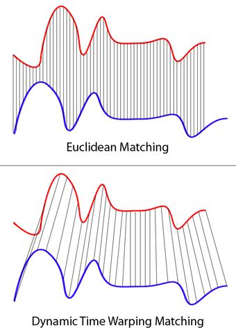
It is difficult to interpret meaning from a bunch of different distances. We can collapse down these distances into a single metric by doing something like taking the square root of the sum of the squared errors. In the Euclidean case the distance is just the sum of the squared distances between the ith point of one series and the ith point of the other series, like we saw in the figure above.
\[D_{Euclidean}(X,Y) = \sqrt{\sum_{i=1}\left(X_{i} - Y_{i}\right)^{2}}\]In the case of DTW we are taking the distance between ith point of one series and jth point of another as defined by the optimal path.
\[D_{DTW}(X,Y) = \sqrt{\sum_{(i,j)\in P}\left(X_{i} - Y_{j}\right)^{2}}\]Where P is the optimal alignment path.
In addition to distance you can also recover the warping path. This allows you to align the two signals and this is where I got into trouble…
Application
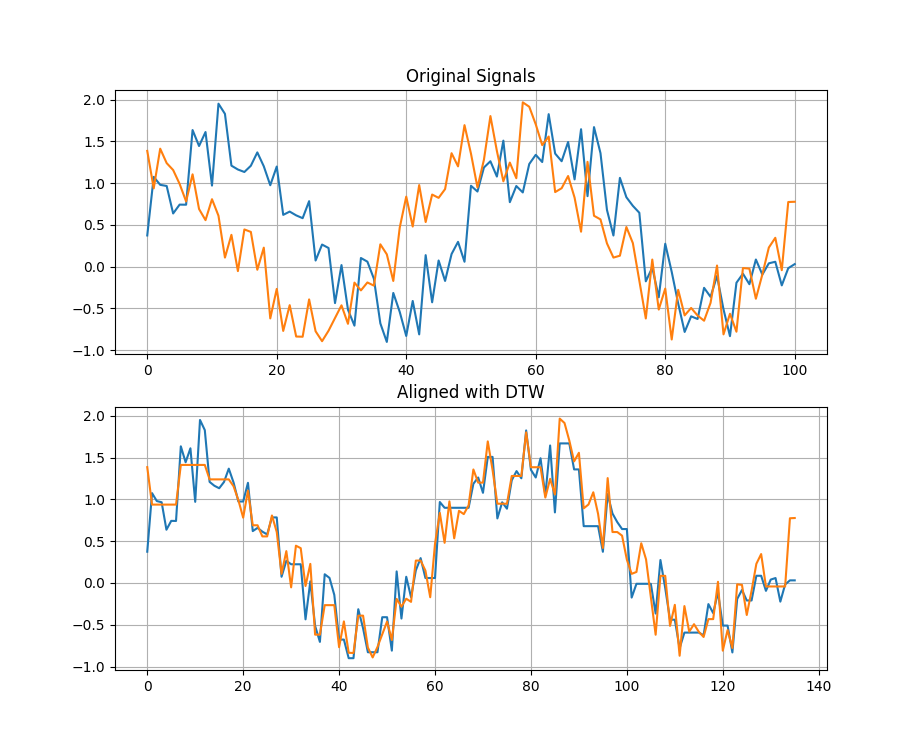
Before implementing the algorithm I wanted to test it on some very simple data to make sure I understand how things worked. I started off with two sine waves, with some added random noise, at different frequencies. You can see from the figure below that DTW does a great job of aligning the signals.
import numpy as np
import matplotlib.pyplot as plt
from tslearn.metrics import dtw_path


np.random.seed(42)
x = np.sin(2 * np.pi * np.linspace(0, 2, 101))
x += np.random.rand(101)

np.random.seed(2)
y = np.sin(2 * np.pi * np.linspace(0.3, 2, 101))
y += np.random.rand(101)
corr1 = np.corrcoef(x, y)
print(f'Correlation before DTW: {corr1[0, 1]:.4f}')

temp, _ = dtw_path(x, y)
x_path, y_path = zip(*temp)
x_path = np.asarray(x_path)
y_path = np.asarray(y_path)
x_warped = x[x_path]
y_warped = y[y_path]

corr2 = np.corrcoef(x_warped, y_warped)
print(f'Correlation after DTW: {corr2[0, 1]:.4f}')

fig, ax = plt.subplots(2, 1)
ax[0].plot(x)
ax[0].plot(y)
ax[0].grid(True)
ax[1].plot(x_warped)
ax[1].plot(y_warped)
ax[1].grid(True)
ax[0].set_title('Original Signals')
ax[1].set_title('Aligned with DTW')
plt.show()
At this point I decided not to try any more simple examples and implement this for the problem I was working on. Before calculating the Pearson’s correlation between each pair of signals, I aligned them using DTW. To my surprise each of the correlations came back very high > 0.6. Some of the signals that originally displayed negative correlation, after alignment, were positively correlated. I knew this was not possible for several combinations of signals. This seemed really odd and I wanted to dig into this further. Since every pair of signals was showing high correlation it seemed that DTW was creating artificial correlation between the signals. To test this I tried the follow steps:
- Generated two random signals
- Calculate the correlation coefficient of the random signals
- Align the signals using DTW
- Re-calculate the correlation coefficient of the aligned signals
import numpy as np
import matplotlib.pyplot as plt
from tslearn.metrics import dtw_path


np.random.seed(42)
x = np.random.rand(100)
np.random.seed(2)
y = np.random.rand(100)

corr1 = np.corrcoef(x, y)
print(f'Correlation before DTW: {corr1[0, 1]:.4f}')

temp, _ = dtw_path(x, y)
x_path, y_path = zip(*temp)
x_path = np.asarray(x_path)
y_path = np.asarray(y_path)
x_warped = x[x_path]
y_warped = y[y_path]

corr2 = np.corrcoef(x_warped, y_warped)
print(f'Correlation after DTW: {corr2[0, 1]:.4f}')

fig, ax = plt.subplots(2, 1)
ax[0].plot(x)
ax[0].plot(y)
ax[0].grid(True)
ax[1].plot(x_warped)
ax[1].plot(y_warped)
ax[1].grid(True)
ax[0].set_title('Original Signals')
ax[1].set_title('Aligned with DTW')
plt.show()
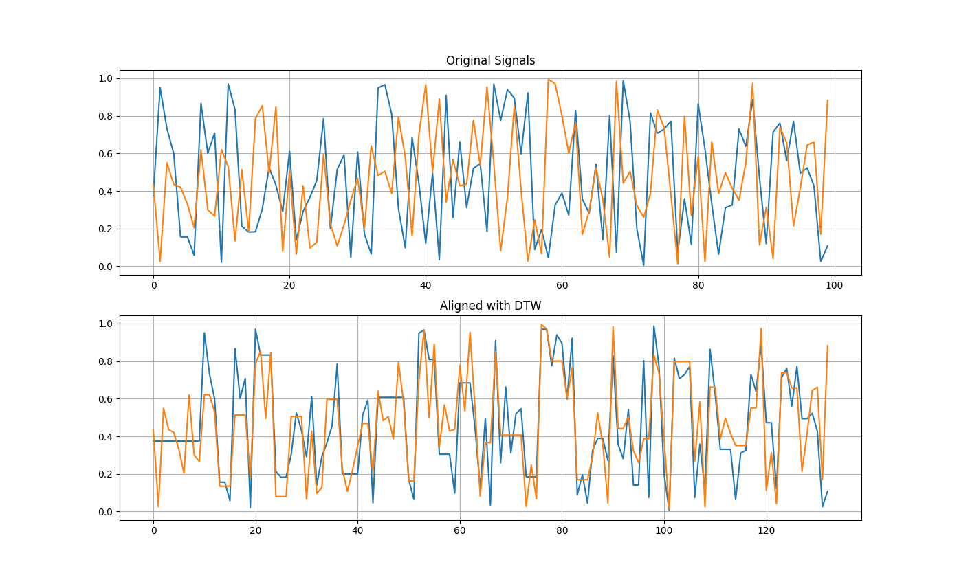
These are two random signals and should have no real correlation, yet after aligning them the correlation jumped to 0.80.
One question that might immediately come to mind is why use the correlation coefficient. Doesn’t DTW have a distance measure?
DTW does return a distance measure between the two signals but it’s difficult to interpret the measure. A distance of 0 means that two signals are perfectly similar or correlated, but what distance corresponds to two signals that should have no correlation?
The correlation coefficient has a nice interpretation, where +1 is total positive linear correlation between two signals, 0 is no linear correlation between two signals, and -1 is total negative linear correlation between two signals.
I think the true benefit of using DTW is in using the distance measure produced by the algorithm, but I don’t believe it’s reasonable to use this metric in an absolute sense. The measure is not normalized, like the correlation coefficient and therefore interpreting the distance measure from DTW by itself is difficult. The distance measure is beneficial when you consider it in a relative sense. For example, if you have a reference signal you can compare multiple signals, using the distance from DTW to determine which signal is most similar to the reference signal. In that case, it’s a relative comparison of the distances between each signal and the reference signal. DTW has found successful applications as a distance measure in clustering algorithms and finding the signal that most closely resembles the reference signal.
Conclusion
Dynamic Time Warping is no doubt a powerful algorithm. But just like any algorithm, be careful how you apply it and make sure it makes sense in the context of the problem you are dealing with.