The purpose of this post is to introduce a new two-step optimizing technique that utilizes Particle Swarm Optimization (PSO) and local numerical optimization. The code for this optimization method can be found here and is a work in progress.
In real-world applications such as hyper-parameter tuning of machine learning models, the function that we are trying to optimize is noisy with many local minimum and maximum values. For example, the image below shows an objective function over a 2-dimensional feature space. In this case, the objective function is the out-of-sample model validation score for a fitted gradient boosted model. The objective function is a function of two hyper-parameters of the model.
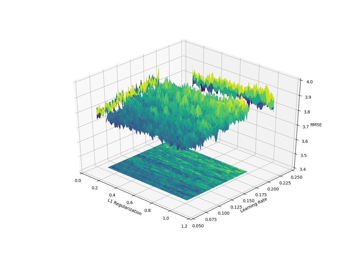
The local noise can skew the search over the global structure. PSO moves candidate solutions (or particles) across the feature space according to the last known best solution of all the particles as a whole and of the individual particles. Where the particle lands on the local variability will help determine the future state of that individual particle as well as all the other particles. The local variability will mask the overall structure of the objective function and either significantly increase the necessary number of iterations necessary to explore the overall structure or make impossible to explore.
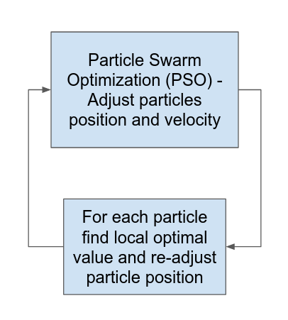
Here we propose a solution to overcome the inconsistencies of local variability. The search over the feature space is divided into two steps. In the first step, we use Particle Swarm Optimization to update a candidate solution within the feature space. After each update, we perform a local optimization within a bounded region of the updated particle’s position. This local optimization ensures that we are searching across the space of the best local solutions. We repeat these two steps for a user-defined number of iterations.
Currently, there are two options for the local optimization scheme. The first option is to perform a Broyden-Fletcher-Goldfarb-Shannon (BFGS) numerical optimization. The second option is to randomly sample within a bounded region of the candidate solution and take the minimum of the objective function within that sample. On the final overall iteration, a BFGS optimization is performed.
The random sampling scheme for the local optimization is computationally cheaper; however, if the most resource-intensive step is in
evaluation of the objective function one should definitely use the BFGS optimization.